A Complete Guide on Stable Diffusion Sampling Methods

Updated on May 31, 2024

Stable Diffusion is a powerful latent diffusion model that has revolutionized the field of generative AI. It allows users to create high-quality images from textual descriptions, enabling a new era of creative expression and exploration. However, the quality and diversity of the generated images heavily depend on the sampling methods employed during the diffusion process.

Sampling methods play a crucial role in guiding the diffusion model towards desired outputs while maintaining coherence and fidelity. They determine how the model navigates the high-dimensional latent space, balancing exploration and exploitation to generate visually appealing and semantically meaningful images.

In this blog post, we will delve into the world of Stable Diffusion sampling methods, exploring their underlying principles, strengths, and weaknesses.

Whether you are a seasoned practitioner or a curious newcomer to the realm of generative AI, understanding Stable Diffusion sampling methods is essential for unlocking the full potential of this groundbreaking technology. By mastering these techniques, you can push the boundaries of creativity, generate captivating visuals, and contribute to the ever-evolving landscape of artificial intelligence.

So, let's embark on this journey together now.

What is Sampling?

If you have learned about how Stable Diffusion works, you must have known that it belongs to a class of deep learning models, i.e. diffusion models. When applying these kinds of models to generate new data, for example, images, they involve two major steps: forward diffusion and reverse diffusion (denoising).

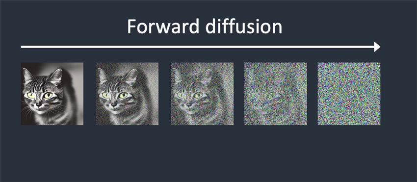
The forward diffusion process starts with a clean input image and gradually adds Gaussian noise to it over multiple steps, following a predefined noise schedule. At each step, a small amount of noise is added to the image, gradually corrupting it until it becomes pure noise at the final step, Like this:

This process can be formulated as a Markov chain, where each step depends only on the previous step, allowing for efficient sampling and closed-form solutions.

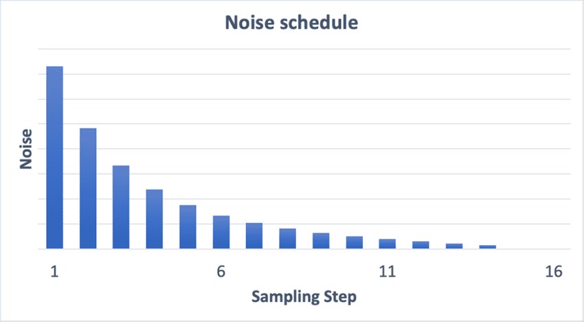
The noise schedule, controlled by a scheduler, determines the amount of noise added at each step, with popular choices like linear, cosine, or other custom schedules.

What about the reverse diffusion process, or called reverse denoising process?

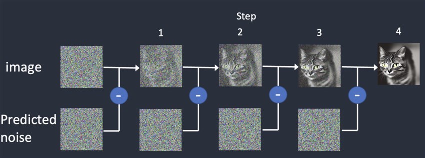
This process starts with a pure noise image from the final step of the forward diffusion process. At each step, the denoising neural network (typically a U-Net) predicts the amount of noise that needs to be removed from the current noisy image.

The sampling method is then coming into this job, which determines how to remove the predicted noise and generates the denoised image for the next step.

Different sampling methods like Euler Ancestral, DPM++ family, PLMS, DDIM, etc. use different strategies and approximations to remove the noise and generate the next denoised image.

This iterative denoising process continues for a fixed number of steps (e.g. 20 steps), with the noise level decreasing at each step according to the predefined noise schedule. In the final step, the model outputs the fully denoised and reconstructed image.

And for this whole process of reverse diffusion, we call it sampling.

The Family of Stable Diffusion Sampling Methods

By far, there have been 31 different Stable Diffusion sampling methods available to its users. In this part, I will try my best to explain them all to you.

Euler-based Samplers: Euler and Euler a

These two are the simplest and fastest sampling methods, based on the Euler method for solving differential equations. They are computationally efficient but may produce noisier or less detailed images compared to more advanced methods.

Mathematically, if we denote the current noisy image as x_t and the predicted noise as ε_theta(x_t, t), then the Euler method to get the denoised image x_(t-1) for the next timestep is given by:

x_(t-1) = x_t - ε_theta(x_t, t)

The key aspects of the Euler method are:

It is the simplest and most straightforward approach, directly subtracting the predicted noise.
It does not use any information from previous denoising steps.
It makes a basic Euler discretization approximation of the underlying diffusion process.

While simple, the Euler method can sometimes produce lower quality images with residual noise compared to more advanced sampling methods. However, it is extremely fast and computationally efficient, making it useful for quickly testing ideas or when generation speed is prioritized over highest possible image quality.

What about the differences between Euler a and Euler?

1. Noise Handling:

Euler: At each denoising step, the Euler method directly subtracts the predicted noise from the current noisy image.
Euler a: In addition to subtracting the predicted noise, Euler Ancestral also adds a small amount of random noise to the image at each step. This makes the denoising trajectory dependent on the specific noise added in previous steps.

2. Consistency:

Euler: The Euler method produces consistent results regardless of the number of denoising steps used, as long as the same seed and prompts are provided.
Euler a: Due to the added random noise, Euler Ancestral can produce significantly different results even with the same seed and prompts, depending on the number of denoising steps used.

3. Image Characteristics:

Euler: Tends to produce more realistic and detailed images, but may sometimes contain residual noise or artifacts.
Euler a: Often generates images with a more dreamy, artistic, or stylized look. It can produce higher-quality results than Euler in some cases, but the output can be less consistent and may require more experimentation to find the optimal number of steps.

4. Computational Efficiency:

Euler: Generally faster and more computationally efficient than Euler Ancestral.
Euler a: Slightly slower than Euler due to the additional noise injection step.

Diffusion Probabilistic Model (DPM) Samplers

DPM++ 2M
DPM++ 2M Karras
DPM++ 2M SDE
DPM++ 2M SDE Karras
DPM++ 2M SDE Exponential
DPM++ 2M SDE Heun
DPM++ 2M SDE Heun Karras
DPM++ 2M SDE Heun Exponential
DPM++ 3M SDE
DPM++ 3M SDE Karras
DPM++ 3M SDE Exponential
DPM++ SDE
DPM++ SDE Karras
DPM++ 2S a
DPM++ 2S a Karras
DPM2 a
DPM2 a Karras
DPM2
DPM2 Karras
DPM fast
DPM adaptive

These samplers are based on Diffusion Probabilistic Models (DPM), which employ probabilistic approaches to estimate and remove noise during the denoising process. They generally produce higher-quality images but are more computationally expensive than Euler-based methods.

DPM Samplers treat the underlying diffusion process as a stochastic differential equation (SDE) that describes the evolution of noise over time. And these samplers employ various probabilistic techniques to estimate and remove the predicted noise during the reverse denoising process, including:

1. Predictor-corrector approach: Many DPM variants use a predictor-corrector approach at each denoising step, where the predictor makes an initial guess, and the corrector refines it using the predicted noise distribution.

2. Probabilistic noise estimation: The denoising neural network predicts the noise distribution present in the current noisy image, which is then used by the DPM sampler to determine the amount of noise to remove.

3. Sampling from the predicted noise distribution: Instead of directly subtracting the predicted noise, some DPM samplers like DPM++ SDE sample from the predicted noise distribution to determine the noise to be removed.

4. Thresholding and distribution matching: Techniques like thresholding and distribution matching are used to ensure that the sampled or denoised images match the training data distribution.

5. Markovian approximations: Variants like DPM++ 2M use second-order Markovian approximations, considering the dependence on previous states of the diffusion process.

By employing these probabilistic techniques, DPM Samplers can better model and approximate the underlying noise distribution, leading to improved image quality and sampling efficiency compared to deterministic numerical methods like Euler.

Among these 21 DPM sampling methods, here are some key sampling algorithms:

1. DPM2 and DPM2 Karras: The original DPM-Solver-2 algorithm, accurate up to the second order of the SDE approximation. The "Karras" variant uses a modified noise scheduler for improved color quality.

2. DPM++ 2M and DPM++ 2M Karras: Improved versions of DPM2, incorporating second-order Markovian approximations for better accuracy. The Karras variant uses the Karras noise scheduler.

3. DPM++ SDE and DPM++ SDE Karras: DPM samplers that model the diffusion process as an SDE, often producing highly detailed and realistic images. The Karras variant is optimized for better performance.

4. DPM-Solver++ and Multistep DPM-Solver++: High-order solvers for the guided sampling of DPMs, addressing instability issues and enabling faster sampling with large guidance scales.

The choice of DPM Sampler variant often involves trade-offs between image quality, generation speed, and computational resources. Generally, DPM++ SDE Karras and DPM++ 2M Karras are considered among the best-performing samplers, particularly at lower sampling steps, but they may be more computationally expensive. And here is more information which can help you make your choice.

The DPM++ variants (e.g., DPM++ 2M, DPM++ SDE) are improvements over the original DPM, incorporating advanced techniques like second-order approximations, stochastic differential equations (SDE), and hybrid deterministic-probabilistic approaches.

The Karras variants (e.g., DPM++ 2M Karras, DPM++ SDE Karras) are optimized versions developed by Timo Karras and his team, known for producing cleaner and more detailed images.

The SDE variants (e.g., DPM++ 2M SDE, DPM++ SDE) use stochastic differential equations to model the diffusion process, often resulting in higher image quality, especially at lower sampling steps.

The Exponential and Heun variants incorporate different numerical approximation methods, which can impact image quality and generation speed.

Heun Sampler

The Heun sampling method is an improvement over the basic Euler method for solving ordinary differential equations (ODEs) and performing denoising during the reverse diffusion process in Stable Diffusion.

Heun's method is a two-stage predictor-corrector method.

At each denoising step, Heun's method first uses the Euler step to predict the denoised image. It then uses the predicted image to estimate the noise again and takes a weighted average of the two noise estimates. This weighted average noise estimate is then subtracted from the current noisy image to obtain the denoised image for the next step.

By incorporating information from both the initial and predicted points, Heun's method achieves higher accuracy compared to the basic Euler method. But the improved accuracy comes at the cost of increased computational complexity compared to Euler.

LMS and LMS Karras Samplers

LMS (Linear Multistep) and LMS Karras are Stable Diffusion sampling methods that employ linear multistep techniques to estimate and remove noise during the reverse denoising process in Stable Diffusion.

Let's be more specific.

LMS (Linear Multistep): LMS is a numerical linear multistep method that combines information from multiple previous denoising steps to estimate and remove noise in the current step.

It uses a different weighting scheme compared to methods like PLMS (Pseudo-Linear Multistep) for combining the information from previous steps.

LMS is known to produce images with a more artistic, stylized, or painterly look, often resembling visual novel backgrounds or paintings.

While it can create good scenery and landscape images, LMS may struggle with generating detailed characters, people, or animals. LMS is generally faster than some other advanced samplers like DDIM but may not match their level of detail and realism.

LMS Karras: LMS Karras is a variant of LMS that incorporates the Karras noise schedule, which aims to improve color quality and image fidelity.

Like LMS, it tends to produce images with a more artistic, painterly, or rough art style.

LMS Karras may suffer from the same weaknesses as LMS when it comes to generating detailed characters or animals.

The key differences between LMS and LMS Karras lie in the noise schedule used (Karras noise schedule for LMS Karras) and the potential for improved color quality in LMS Karras. However, both methods are known for their artistic, stylized outputs and may not be the best choice for highly detailed or photorealistic images, especially when it comes to characters or animals.

DDIM (Denoising Diffusion Implicit Models) Sampler

DDIM was one of the first sampling methods designed specifically for diffusion models like Stable Diffusion. It is based on the idea of implicit discretization of the underlying diffusion process. It uses an implicit numerical solver to approximate the denoising step, rather than explicit discretization methods like Euler.

At each denoising step, DDIM solves a fixed-point equation iteratively to estimate the amount of noise to remove from the current noisy image. This involves combining the final denoised image, the current image direction, and random noise using specific formulas derived from the implicit discretization.

DDIM can produce high-quality, detailed images but generally requires a higher number of sampling steps compared to some newer methods like DPM++ SDE Karras.

It is known for its ability to achieve photorealistic results and is often recommended for generating photorealistic images.

However, DDIM can be slower than some other samplers like Euler or DPM++ variants, especially at higher sampling steps.

While DDIM was widely used in the original Stable Diffusion v1 release, it is now considered somewhat outdated and has been largely superseded by newer samplers like DPM++ SDE Karras, which can achieve similar or better quality with fewer sampling steps.

PLMS (Pseudo Linear Multistep Sampling) Sampler

PLMS is based on a linear multistep numerical method for solving ordinary differential equations.

It combines information from multiple previous denoising steps using a specific weighting scheme to estimate the noise to be removed in the current step.

PLMS makes the approximation that the underlying diffusion process can be locally linearized over multiple steps. This allows for a pseudo-linear estimation of the noise, rather than relying on probabilistic modeling like in DPM samplers.

LCM (Latent Consistency Model) Sampler

One of the primary techniques employed by LCM is latent space refinement. It utilizes the latent space of pre-trained autoencoders to refine the guided diffusion model. The focus is on maintaining the trajectory consistency of generated samples in this latent space, ensuring that the generated images remain coherent and aligned with the pre-trained autoencoder's representations.

Another key aspect of LCM is its ability to generate high-quality images in a single step of inference. While designed for single-step generation, in practice, LCM adds noise back to the image and denoises again, repeating this process for a few steps (typically 1-4 steps). This iterative approach, combined with the latent space refinement, allows for efficient synthesis of high-resolution images with fewer sampling steps compared to traditional methods.

Furthermore, LCM can serve as a plug-and-play neural ODE solver, predicting solutions in the latent space without the need for iterative solving through numerical ODE solvers. This approach contributes to the efficient sampling capabilities of LCM, enabling the synthesis of high-quality images with reduced computational requirements.

One of the notable strengths of LCM is its versatility. It can be directly applied to various fine-tuned Stable Diffusion models and LoRA models without requiring additional training. This makes LCM a universal acceleration module, supporting various image generation tasks and models within the Stable Diffusion framework.

Additionally, LCM enforces a latent consistency constraint during the sampling process. This constraint ensures that the generated samples remain consistent with the pre-trained autoencoder's latent space, helping to maintain the quality and coherence of the generated images.

Restart Sampler

At its core, the Restart method alternates between two subroutines: a Restart forward process that adds a substantial amount of noise, akin to "restarting" the original backward process, and a Restart backward process that runs the backward ordinary differential equation (ODE).

This forward-backward cycle of adding noise and running the backward ODE is repeated K times within a predefined time interval [tmin, tmax]. The key innovation lies in the separation of stochasticity and drifts. Unlike previous stochastic differential equation (SDE) methods that add small single-step noise, the Restart forward process introduces a significantly larger amount of noise. This amplifies the contraction effect on accumulated errors from previous steps, allowing for more effective self-correction compared to traditional ODE or SDE methods.

UniPC (Unified Predictor-Corrector) Sampler

The UniPC sampling method applies a unique approach to accelerate and improve the sampling process across various probabilistic models. At its core, UniPC employs a unified predictor-corrector framework consisting of two main components: a unified predictor (UniP) and a unified corrector (UniC).

Both the UniP predictor and UniC corrector share a unified analytical form, allowing them to support arbitrary orders of accuracy. This unified form enables UniPC to adapt to different levels of precision without requiring additional model calculations, making it a flexible and efficient framework. UniPC aims to achieve high-order accuracy in its predictions and corrections, enabling faster convergence compared to previous methods. By increasing the order of accuracy, UniPC can remarkably improve sampling quality, especially when using an extremely low number of steps.

One of the key strengths of UniPC is its model-agnostic approach. It is designed to support both pixel-space and latent-space diffusion probabilistic models (DPMs), making it applicable to unconditional and conditional sampling tasks, as well as noise prediction models and data prediction models. This versatility allows UniPC to be applied across a wide range of probabilistic models, including image synthesis tasks using pre-trained models like Stable Diffusion.

A significant advantage of UniPC is its ability to enable swift and high-quality sampling. By converging faster due to its high-order accuracy, UniPC can significantly reduce the required number of sampling steps compared to previous methods, leading to accelerated image generation while maintaining or improving image quality.

Furthermore, UniPC is a training-free framework, meaning it does not require additional training or fine-tuning of the underlying diffusion model. It can be directly applied to pre-trained models, acting as a plug-and-play acceleration module for efficient image generation. This training-free nature makes UniPC a versatile and practical solution for accelerating sampling across various probabilistic models, including Stable Diffusion.

How to Choose Stable Diffusion Sampling Methods

The choice of sampling method depends on the desired trade-off between image quality, generation speed, and computational resources. Generally, the DPM++ variants, especially those with "SDE" and "Karras" optimizations, are considered among the best-performing samplers, particularly at lower sampling steps. However, they may be more computationally expensive.

For high-quality image generation with reasonable speed, DPM++ 2M Karras, DPM++ SDE Karras, and Euler a (Euler Ancestral) are often recommended choices. Euler and DPM fast can be used for faster generation when speed is prioritized over image quality.

It's important to note that the optimal sampling method may vary depending on the specific use case, prompt, and desired image characteristics. Experimentation and benchmarking with different methods can help determine the best fit for a particular scenario.

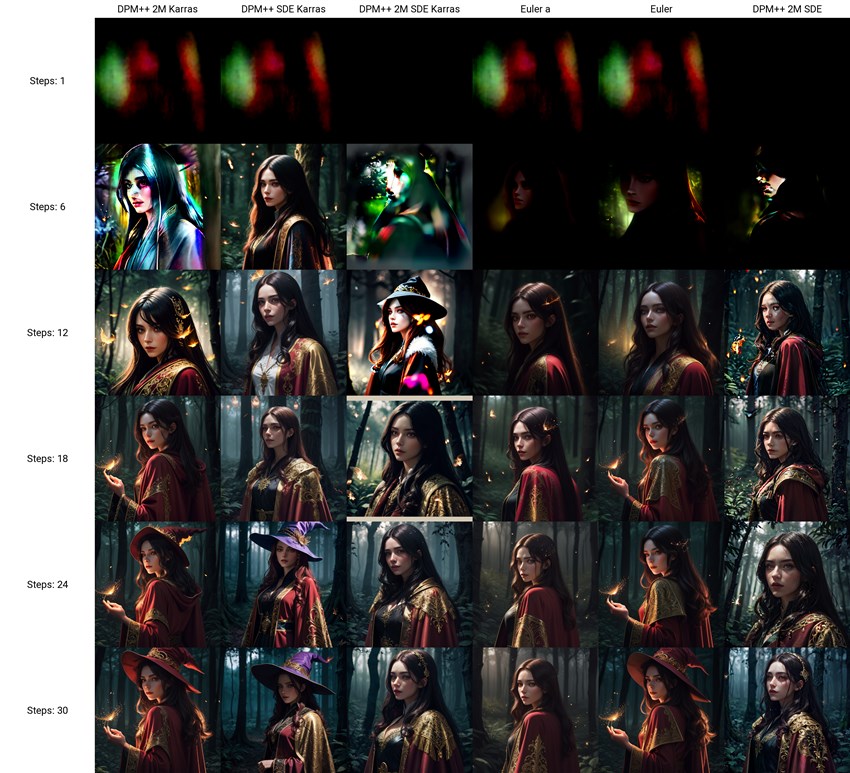
Still feel confused? No worries. Here is a simple feature in the AUTOMATIC1111 Web UI which can help you easily make your decision about which sampling method you should go for. And it is the X/Y/Z plot.

The X/Y/Z plot is a powerful tool that allows you to test and visualize the impact of varying multiple parameters or settings on the generated images. It enables you to explore how different combinations of values affect the output, providing valuable insights for fine-tuning and optimizing your image generation process.

And here is how to use it,

Step 1. Run AUTOMATIC1111 Web UI on your computer, input your prompt, both the positive and negative ones, and set other parameter values to what you prefer, such as Checkpoint, VAE, Clip skip, Textual Inversion, LoRA, width and height, CFG Scale, batch count and batch size, etc.

Step 2. Now scroll down to the bottom and find the Script dropdown menu.

Step 3. Click it and choose the X/Y/Z plot. In the X type, find and choose Sampler; In the Y and Z types, find and choose other values which you want to test. Here on this guide, we choose the Steps to show you how it works.

Step 4. Lastly, head back to the beginning and click the Generate button. Stable Diffusion will start the creation and give you the comparison image. And here is what I got based on my settings.

Stable Diffusion X/Y/Z grid test for Sampling Methods and Steps

Make Your 512p/1024p AI Arts Bigger and Clearer